How to Use Conditional Formatting in Google Sheets

 

Summary.

Conditional Formatting allows us to change the style of a cell in Google Sheets when certain conditions are met or changed. Almost all of our Dashboards use Conditional Formatting to change the color of the Dashboard. In fact, our very first Dashboard, Neutral Loan Tracker uses Conditional Formatting to change the Theme of the Dashboard!

In this tutorial, we will cover 3 common questions.

• Question #1 - Where to find Conditional Formatting in the Tools Menu?
• Question #2 - What can be Conditionally Formatting?
• Question #3 - Can Conditional Formatting be changed?

Question #1 - Where to find Conditional Formatting in the Tools Menu?

Conditional Formatting is located in Format > Conditional formatting. 

Figure 1. Conditional Formatting Menu Location

After you click on the menu, a panel will open up on the right hand side. If you have not created any conditions, the panel will be empty. But if you have, you'll see all conditions created on that cell. 

To view Conditional Formatting for a range, all you have a to do is select the range!

Figure 2. Conditional Formatting Panel

Question #2 - What can be Conditionally Formatting?

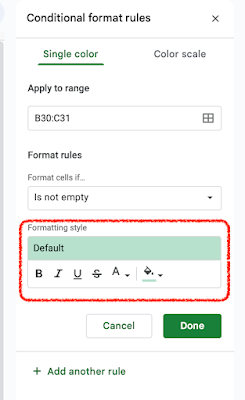
Anything that can be normally style on a cell can be accomplished using Conditional Formatting. This includes changing fonts, cell background, adding bold, adding underlines, adding italics, adding strikethrough, and changing font color.

Figure 3. Available Formatting Style Options

To create a new Conditional Formatting, click on "Add Another Rule". 

Figure 4. Creating a new Rule

The Panel will open up a new page where you can select the range, the format rules, and the formatting style. 

Figure 5. Conditional Format Rules

There are currently 18 predefined rules that will cover most conditions in Google Sheets. However if you need to create a custom rule, the 19th option is "Custom formula is". 

 "Custom formula is " will allow us to create more complex conditions using Google Sheets plethora of functions such as IF() functions, MATCH(), etc. Most of our Dashboards uses the Custom Formula rules to achieve more sophisticated conditions such as strikethroughs when a checkbox is clicked, cell background color changes when a dropdown is changed, and many more. 

Here is one custom formula rule that is fairly easy to understand. This rule will change the background color of range, V5:V38 when cell C27 (a dropdown) is equal to "Monochromatic".

Figure 6. Custom Formula Rule

Question #3 - Can Conditional Formatting be Changed?

After a rule is created, you can edit it or delete it altogether. Additionally, you can create an infinite amount of rules on a single cell.

Figure 7. Multiple Custom Formula Rules

If you have questions or suggestions, please comment below. In the meantime, Happy Planning!